Features and Usages

Spreadsheet User Interface Overview

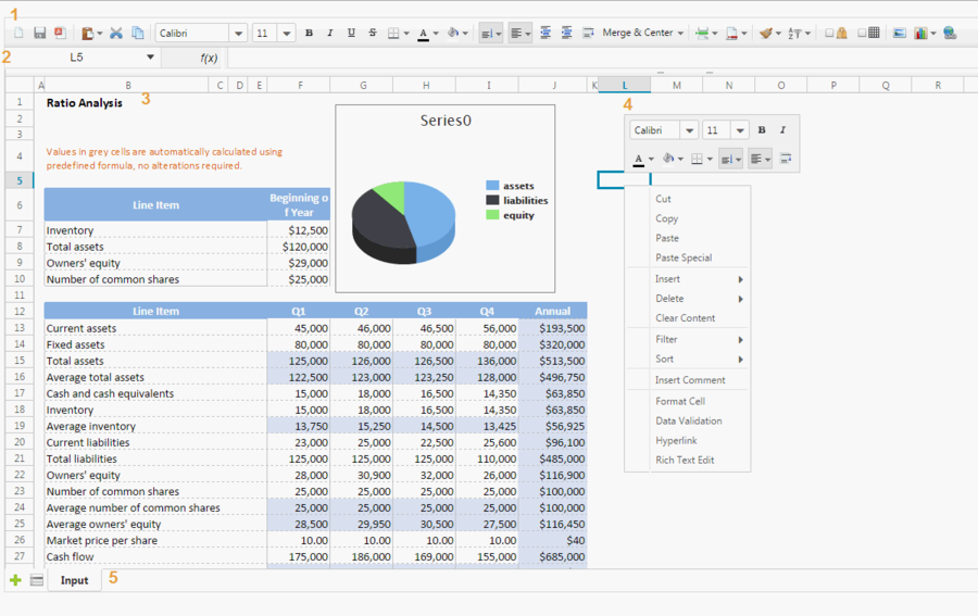
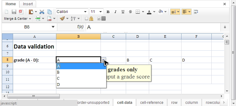
Above is a screenshot of ZK Spreadsheet's user interface, each section is introduced in the following:

1. Toolbar

   The toolbar contains all commonly-used functions including setting cell's style, alignment, border, background color, font, font color, merging (and unmerging) of cells, sorting, auto filter, protection and grid line visibility. It has 2 tabs, another tab is used to insert charts, images, and hyperlinks for web page and email address:

   

   The 3 leftmost buttons, "New Book", "Save Book", and "Export to PDF", are not built-in functions. You have to implement them by yourself.

2. Formula bar

   It displays editing text or formula of current selected cell and can be used to enter or edit a formula or data.

3. Sheet Area

   It displays the content of current selected sheet, and you usually perform most editing operations in this area.

4. Context menu

   Right clicking on a cell, a column header, or a row header pops up a context menu. It contains most options of the toolbar and works like a shortcut.

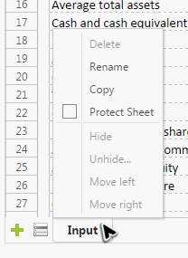
5. Sheet bar

   A list of all sheets in this book. You can navigate to any sheet by clicking on it. Click can add a new sheet. Right clicking on a sheet pops a context menu and it allows you to delete, rename, protect, and move the clicking sheet.

   

Supported Hotkeys

Hotkey	Action
Ctrl+B	bold
Ctrl+C	copy
Ctrl+I	italic
Ctrl+U	underline
Ctrl+V	paste
Ctrl+X	cut
Ctrl+Y (EE only)	redo
Ctrl+Z (EE only)	undo
Delete	clear content
Esc	clear copy/cut clipboard

Usage

The following sections will introduce usages of some noticeable features which are all Available in ZK Spreadsheet EE only.

Special Paste

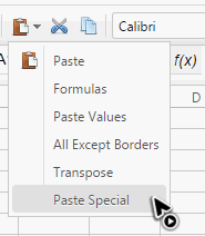
In addition to normal pasting, Spreadsheet also provides other special pasting options on the toolbar.

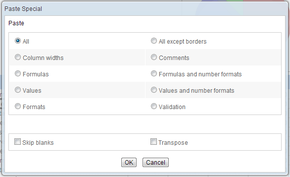
You can select "Paste Special" to access all available pasting options in a dialog.

Custom Sort

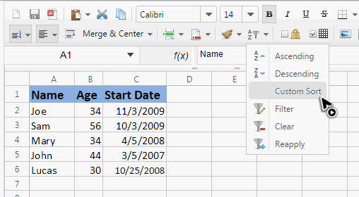
The "Ascending" and "Descending" function can sort data by only one column but "Custom sort" can sort data by multiple columns.

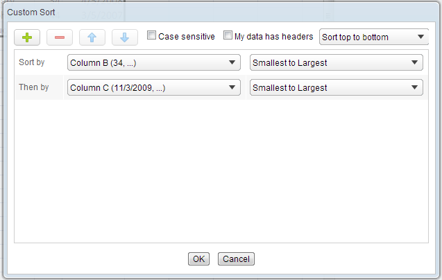
After selecting "Custom sort" on the toolbar, a dialog appears. You can add sorting criteria to 3 columns at the most. If your data includes column headings, make sure the "My data has headers" option is checked.

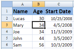
The sorting result of criteria above:

Filter

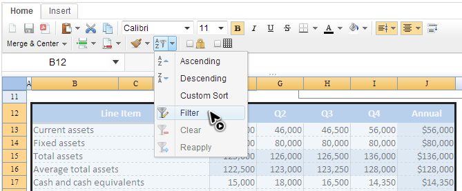
The Filter can screen out data you don't want displayed quickly and easily. We usually select the cells we want to filter first and select "Filter" on the toolbar.

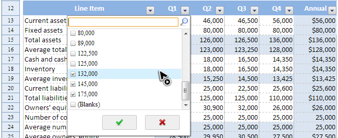
Then each column will have a drop-down button. Click the drop-down button to select data to filter.

Those rows that contain the unchecked item will not appear in the original table unless you check them back.

If you insert more data after applying a filter, you can select "Reapply" on the toolbar to apply same criteria to new data.

Auto Fill

Auto fill is a handy feature to fill cells with data using a particular pattern based on selected cells. Text will be copied and numbers and dates will be increased (or decreased).

To use this, You should select one or more cells and drag the fill handle across or down the cells that you want to fill.

Fill cells after dragging right.

Format Cell

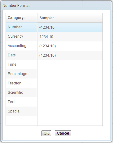
A context menu appears when right clicking a cell, "Format Cell" provides 10 different categories with total of 47 formats to apply on cells.

Validation

Spreadsheet can read your validation settings in an Excel file and show hints and validate inputs for you. (Spreadsheet OSE will ignore validation settings.)

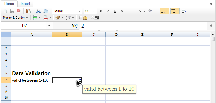
When you select a cell with validation settings, Spreadsheet will display input message aside the cell.

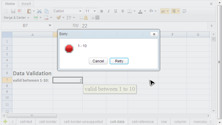
If you enter invalid data, Spreadsheet will prompt you with the error message you set in the Excel file.

If your validation criteria comes from a range of data, you can input that cell via a drop-down list.

Protection

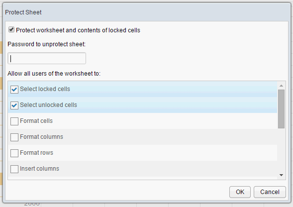
If you enable "Protect Sheet" for a sheet in Excel, Spreadsheet will keep this setting when reading the Excel file, hence, when you edit a protected sheet, you will receive an alert message on the top left-hand corner.

All source code listed in this book is at Github.